Cancer Genome in a Bottle (SVs)

This tutorial walks through loading data from the Cancer Genome in a Bottle (C-GIAB) project into JBrowse 2 and using several view types to inspect the supplied benchmark structural variant (SV) and copy-number variant (CNV) calls. The dataset is HG008, a pancreatic ductal adenocarcinoma (PDAC) cell line with matched tumor and normal tissue, sequenced with PacBio HiFi long reads. The project also publishes a phased de novo assembly of the tumor genome, which is particularly well-suited to JBrowse 2's synteny and dotplot views.

C-GIAB ships several complementary assays beyond bulk sequencing — karyotyping, directional genome hybridization (DGH), and other cytogenetic characterizations — which together informed the high-quality benchmark call sets used here. This tutorial does not load those auxiliary datasets, but the NIST C-GIAB page is the place to find them, along with McDaniel et al. 2025 for the methods behind the dataset.

The general SV-visualization concepts used below are documented in the SV visualization guide and the SV inspector guide. This tutorial focuses on the data-loading workflow and a few worked examples.

What you need

This tutorial assumes you are setting up a JBrowse 2 instance on an Apache 2 HTTP server on Ubuntu or Debian Linux, but the data-preparation steps work on any platform.

You will need:

• A Linux machine with HTTP access (either a public URL or http://localhost)
• Approximately 1 TB of free disk space — the BAM/CRAM files are large
• At least 32 GB of RAM for the minimap2 alignment step (you can downsize the machine after data prep is done; a 2 GB instance is sufficient to host the finished site)
• The following command-line tools, with versions tested at the time of writing in parentheses:
  • JBrowse CLI (@jbrowse/cli v3.6.5)
  • Node.js (v24.1.0)
  • tabix (v1.21)
  • samtools (v1.21)
  • minimap2
  • megadepth (v1.2.0)

A script with all of the data-preparation commands below is available as a gist.

Install JBrowse 2 with Apache 2

Install system dependencies and the JBrowse CLI:

export OUT=/var/www/html/jbrowse2
sudo apt-get update
sudo apt-get install nodejs wget apache2 tabix samtools minimap2
sudo service apache2 start

# confirm node.js >= v18 is installed
node --version
sudo npm install -g @jbrowse/cli

# confirm the jbrowse CLI is installed
jbrowse --version

# download and unzip the latest JBrowse 2, then move it into the web root
jbrowse create tmpdir
sudo mv tmpdir $OUT

jbrowse create downloads the latest jbrowse-web.zip from the GitHub releases page and unzips it. See the web quickstart for more on basic JBrowse 2 setup.

Load the human reference

The C-GIAB project uses a specific build of GRCh38 with decoys and several masked regions. The build is not critical to the visualization itself, but it is important to use the same reference when converting the BAM files to CRAM in later steps.

# download and prepare the GRCh38 build used by the C-GIAB project
curl https://ftp-trace.ncbi.nlm.nih.gov/ReferenceSamples/giab/release/references/GRCh38/GRCh38_GIABv3_no_alt_analysis_set_maskedGRC_decoys_MAP2K3_KMT2C_KCNJ18.fasta.gz > GRCh38_GIABv3.fa.gz
gunzip GRCh38_GIABv3.fa.gz
samtools faidx GRCh38_GIABv3.fa
jbrowse add-assembly GRCh38_GIABv3.fa --out $OUT --load copy

# add NCBI RefSeq gene annotations
jbrowse add-track https://jbrowse.org/ucsc/hg38/ncbiRefSeq.gff.gz \
  --indexFile https://jbrowse.org/ucsc/hg38/ncbiRefSeq.gff.gz.csi --out $OUT

Load the C-GIAB benchmark SV and CNV calls

Load the V0.4 HG008-T draft benchmark SV calls (VCF) and CNV calls (BED). The BED file ships without a header, so we prepend one to give each column a name:

# C-GIAB benchmark SVs (VCF)
jbrowse add-track https://ftp-trace.ncbi.nlm.nih.gov/ReferenceSamples/giab/data_somatic/HG008/Liss_lab/analysis/NIST_HG008-T_somatic-stvar-CNV_DraftBenchmark_V0.4-20250714/GRCh38_HG008-T-V0.4_somatic-stvar_PASS.draftbenchmark.vcf.gz \
  --out $OUT --category "Variant calls"

# C-GIAB benchmark CNVs (BED, with custom header prepended)
(echo "#chr"$'\t'"start"$'\t'"end"$'\t'"total_copy_number"$'\t'"hap1_copy_number"$'\t'"hap2_copy_number"$'\t'"name" \
  && curl https://ftp-trace.ncbi.nlm.nih.gov/ReferenceSamples/giab/data_somatic/HG008/Liss_lab/analysis/NIST_HG008-T_somatic-stvar-CNV_DraftBenchmark_V0.4-20250714/GRCh38_HG008-T-V0.4_somatic-CNV_PASS.draftbenchmark.calls.bed) \
  > GRCh38_HG008-T-V0.4_somatic-CNV_PASS.draftbenchmark.calls.bed
jbrowse add-track GRCh38_HG008-T-V0.4_somatic-CNV_PASS.draftbenchmark.calls.bed \
  --out $OUT --category "Variant calls" --load move

Convert tumor and normal reads to CRAM, and compute coverage

The tumor and normal BAM files at the C-GIAB FTP are large and slow to access remotely, and lack MD tags (which JBrowse uses to display SNP positions without re-fetching the reference). We download them with samtools view, write them out as CRAM, and compute whole-genome coverage with megadepth:

# convert remote BAM files to local CRAM files
# note: this downloads >200 GB of data
samtools view -@8 ftp://ftp-trace.ncbi.nlm.nih.gov/ReferenceSamples/giab/data_somatic/HG008/Liss_lab/PacBio_Revio_20240125/HG008-N-P_PacBio-HiFi-Revio_20240125_35x_GRCh38-GIABv3.bam \
  --write-index -o HG008-N-P_PacBio-HiFi-Revio_20240125_35x_GRCh38-GIABv3.cram -T GRCh38_GIABv3.fa
samtools view -@8 ftp://ftp-trace.ncbi.nlm.nih.gov/ReferenceSamples/giab/data_somatic/HG008/Liss_lab/PacBio_Revio_20240125/HG008-T_PacBio-HiFi-Revio_20240125_116x_GRCh38-GIABv3.bam \
  --write-index -o HG008-T_PacBio-HiFi-Revio_20240125_116x_GRCh38-GIABv3.cram -T GRCh38_GIABv3.fa

# fetch the megadepth executable
wget https://github.com/ChristopherWilks/megadepth/releases/download/1.2.0/megadepth
chmod +x megadepth

# compute coverage and add both the CRAM and bigWig to the JBrowse config
# note: this loop takes 10-15 minutes per CRAM
for i in *.cram; do
  ./megadepth $i --bigwig
  jbrowse add-track $i --out $OUT --category "Reads" --load move
  jbrowse add-track $i.all.bw --out $OUT --category "Coverage" --load move
done

Align the phased tumor assembly to GRCh38

The C-GIAB project provides a phased de novo assembly of HG008-T (two haplotypes), produced with verkko. Aligning both haplotypes against GRCh38 with minimap2 gives us PAF files that JBrowse can render in the synteny and dotplot views — these are particularly helpful for complex SVs that are hard to read directly off the alignment track.

# download the phased assembly (two haplotypes)
curl https://ftp-trace.ncbi.nlm.nih.gov/ReferenceSamples/giab/data_somatic/HG008/Liss_lab/analysis/Verkko_assemblies_05162024/HG008T/HG008T_verkko_v2.2.1_herro_corrected/PBhifi+20kbBCMhifi_UL_ONTq26_herro/assembly.haplotype1.fasta > HG008T.hap1.fa
curl https://ftp-trace.ncbi.nlm.nih.gov/ReferenceSamples/giab/data_somatic/HG008/Liss_lab/analysis/Verkko_assemblies_05162024/HG008T/HG008T_verkko_v2.2.1_herro_corrected/PBhifi+20kbBCMhifi_UL_ONTq26_herro/assembly.haplotype2.fasta > HG008T.hap2.fa

# load both haplotypes as JBrowse assemblies
samtools faidx HG008T.hap1.fa
samtools faidx HG008T.hap2.fa
jbrowse add-assembly HG008T.hap1.fa --load copy --out $OUT
jbrowse add-assembly HG008T.hap2.fa --load copy --out $OUT

# align each haplotype to GRCh38 with minimap2
# note: each command takes about 20 minutes
minimap2 -t8 -cx asm5 GRCh38_GIABv3.fa HG008T.hap1.fa > HG008T.hap1.paf
minimap2 -t8 -cx asm5 GRCh38_GIABv3.fa HG008T.hap2.fa > HG008T.hap2.paf

# load the alignments as synteny tracks
jbrowse add-track HG008T.hap1.paf -a HG008T.hap1,GRCh38_GIABv3 --out $OUT --load copy
jbrowse add-track HG008T.hap2.paf -a HG008T.hap2,GRCh38_GIABv3 --out $OUT --load copy

The -c flag asks minimap2 to emit base-level CIGAR strings, which encode the position of insertions and deletions in the alignment. The -x asm5 preset sets parameters for same-species assembly-to-assembly alignment. The order of assemblies passed to add-track -a query,ref must match the order in the minimap2 command — see the linear synteny view guide.

Walkthroughs

Once your JBrowse 2 instance is live, you can explore the loaded data using three complementary approaches: the SV inspector for whole-genome triage, the linear genome view for read-level detail at small-to-medium SVs, and the dotplot/synteny views for chromosome-scale rearrangements in the assembly.

Walkthrough: a chr3–chr13 translocation

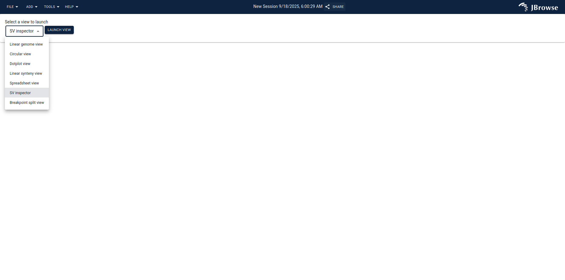
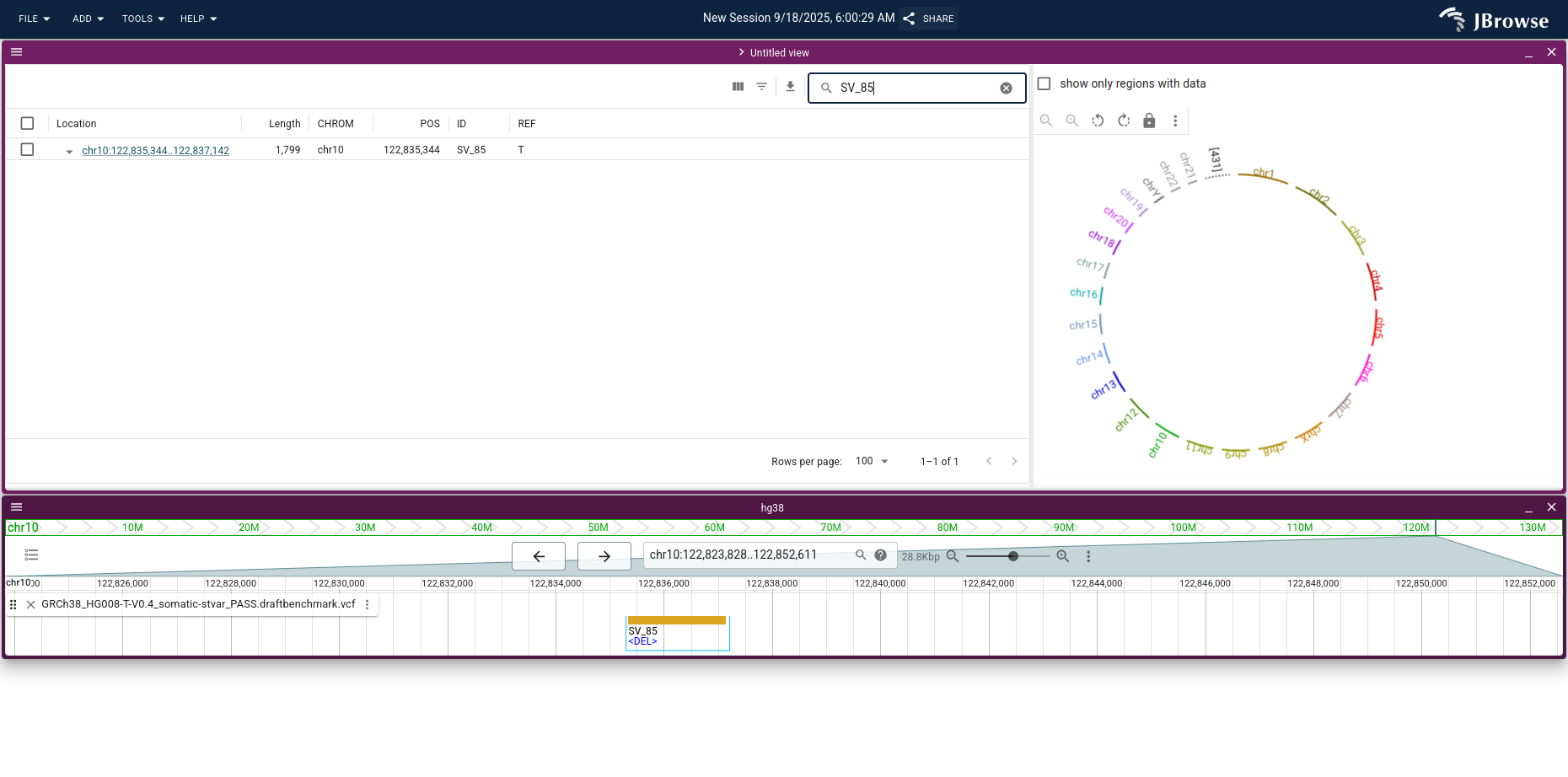
Open http://yourhost.com/jbrowse2/ in a web browser. From the start screen, launch the SV inspector.

The start screen with the SV inspector launcher.

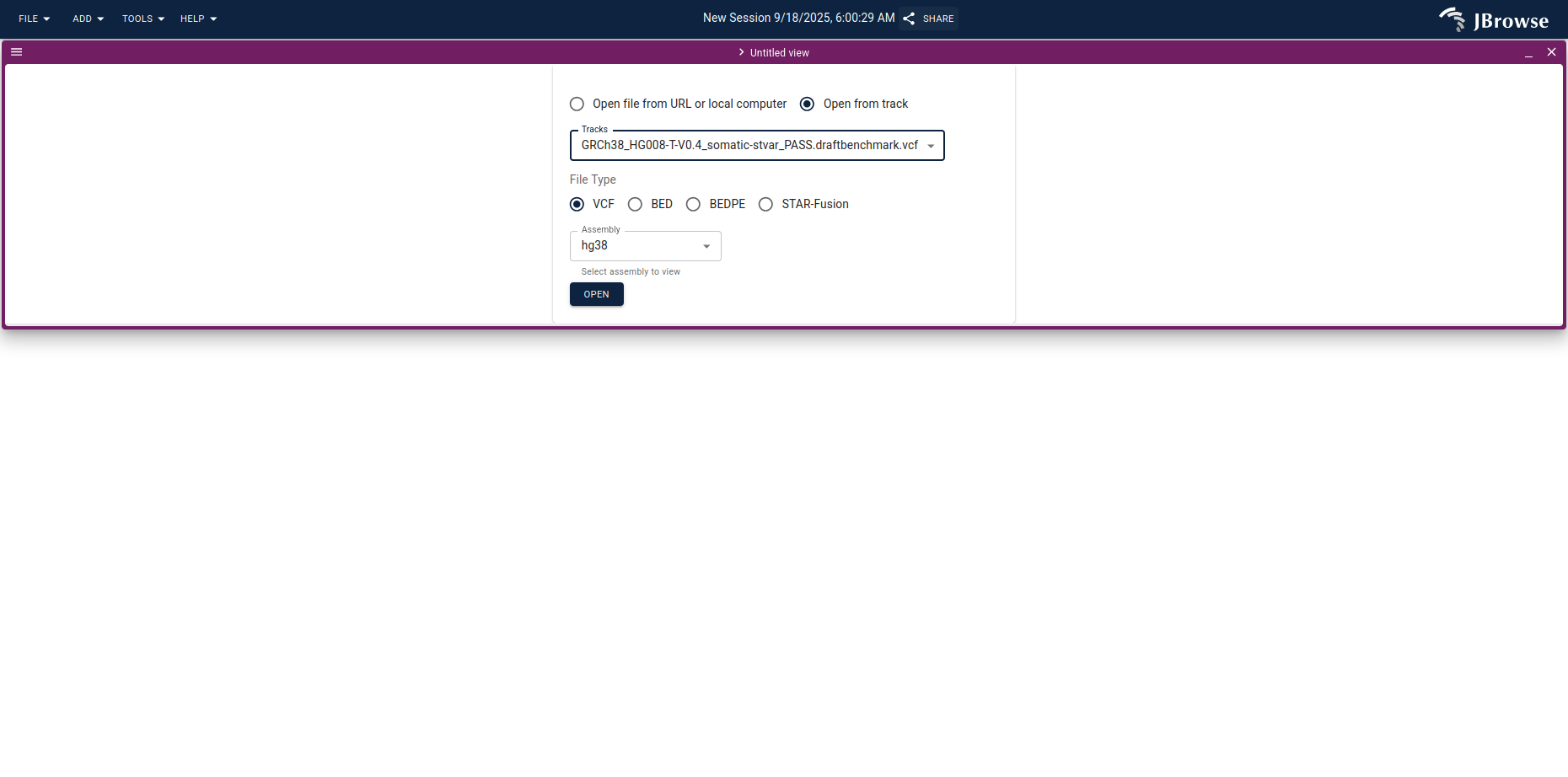
Use Open from track to pick the C-GIAB benchmark VCF you loaded earlier.

The Open from track dialog with the C-GIAB SV benchmark VCF selected.

The result is a combined data table and circular overview of the SV calls.

The SV inspector showing the benchmark VCF as a circular overview and a table.

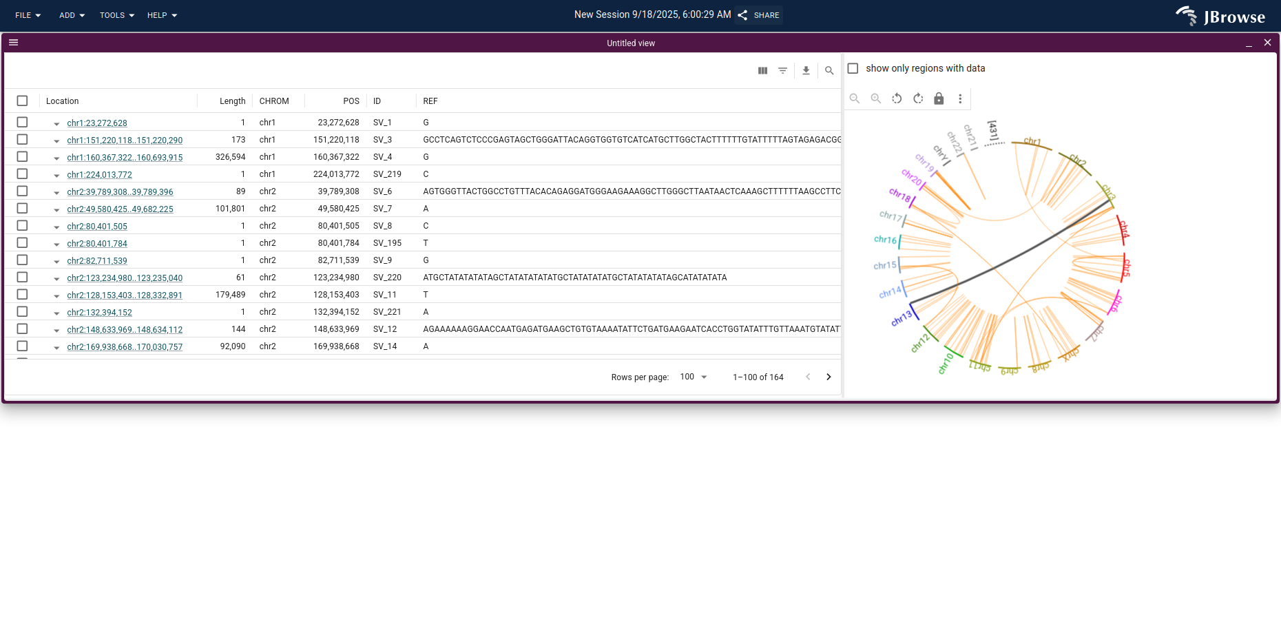
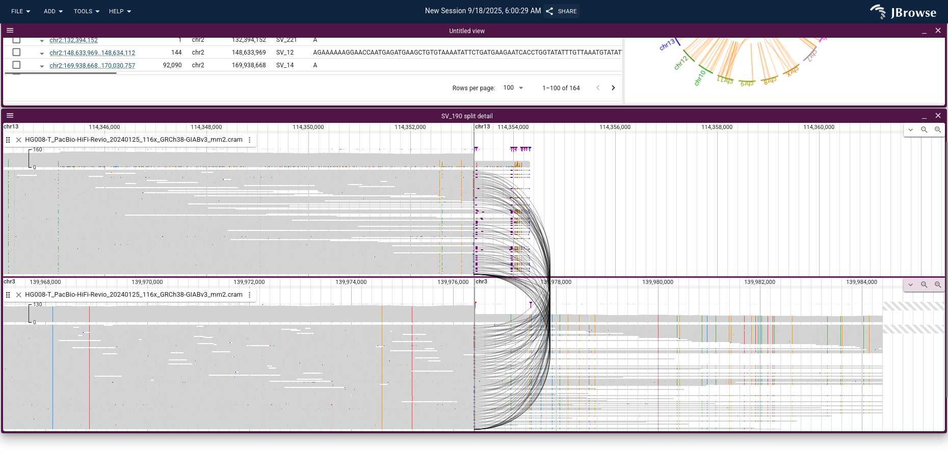
Clicking the chord that connects chr3 and chr13 launches a breakpoint split view; opening the tumor PacBio HiFi reads on each panel and switching to compact mode highlights the supporting split reads as black splines connecting the two chromosomes.

Clicking the chord joining chr3 and chr13 opens a breakpoint split view. Black splines connect tumor PacBio HiFi reads that partially map to each chromosome, suggesting a fusion or translocation.

For the SV inspector workflow itself (filtering the table, search, configuring the circular overview), see the SV inspector guide.

Walkthrough: a small deletion in CUZD1

For small to medium SVs, the linear genome view is usually all you need. Use the search (magnifying glass) button in the SV inspector to find a specific call — for example, SV_85, a heterozygous deletion that affects two exons of the CUZD1 gene.

The SV inspector after searching for SV_85 — clicking the row opens a new linear genome view.

Opening the gene annotations and the tumor PacBio HiFi reads, switching the reads to compact mode, and applying Sort by → Base pair with the deletion centered shows the deletion (View menu → Show center line is helpful for placing the center line on the breakpoint).

After opening the gene annotations and tumor PacBio HiFi reads, displaying reads in compact mode, and sorting by base pair with the deletion in the center. The deletion removes two CUZD1 exons and is heterozygous.

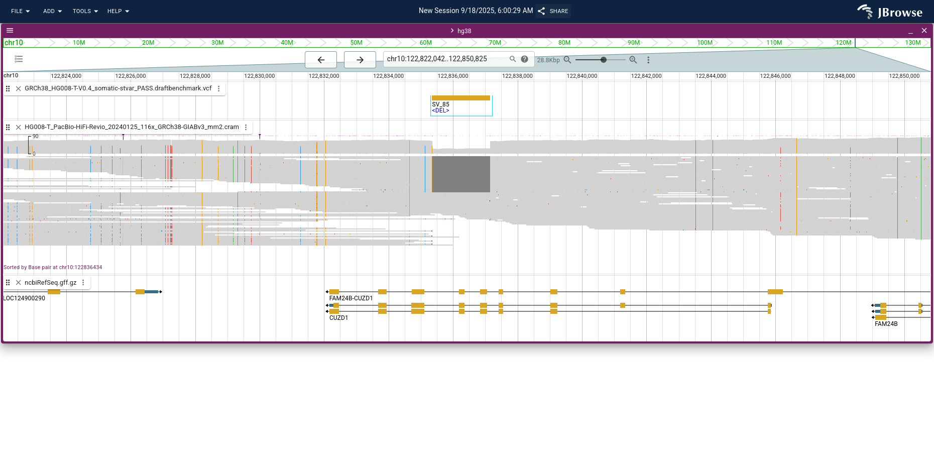
For background on SV signals in the alignments track, see the SV visualization guide.

Walkthrough: CNVs from coverage

Loading raw reads across very large regions is impractical, but whole-genome coverage stored as a bigWig is fast at any zoom level. From the linear genome view start screen, click Show all regions in assembly to open every chromosome at once.

The linear genome view start screen with the 'Show all regions' button.

Open the tumor and normal bigWigs as a multi-bigwig track for direct comparison.

A multi-bigwig track with tumor and normal coverage across all chromosomes.

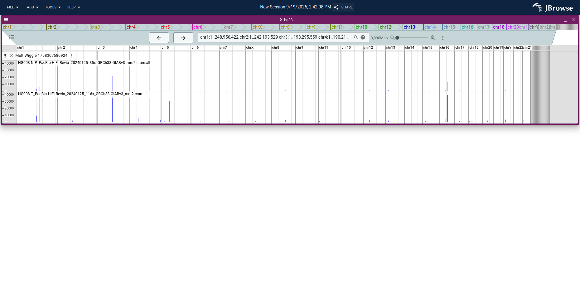
Apply a manual score limit (Track menu → Score → Set min/max score) to cap the y-axis at, e.g., 300.

After applying a manual score limit of 300.

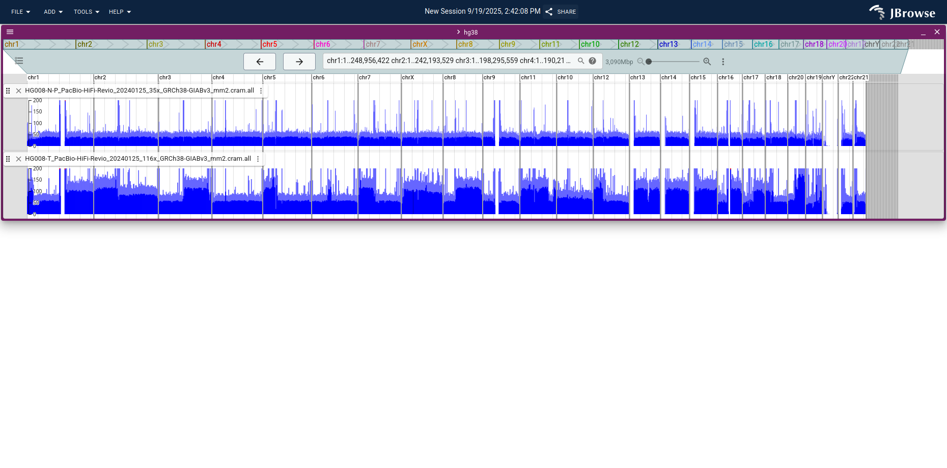
Switch Fill mode → No fill for a clearer line-style trace, zoom into a region of interest, and open the benchmark CNV BED track to check whether coverage changes line up with the called CNVs.

After switching to no-fill mode, zooming into chromosome 5, and opening the benchmark CNV BED track — orange boxes mark individual CNVs and clicking them shows feature details.

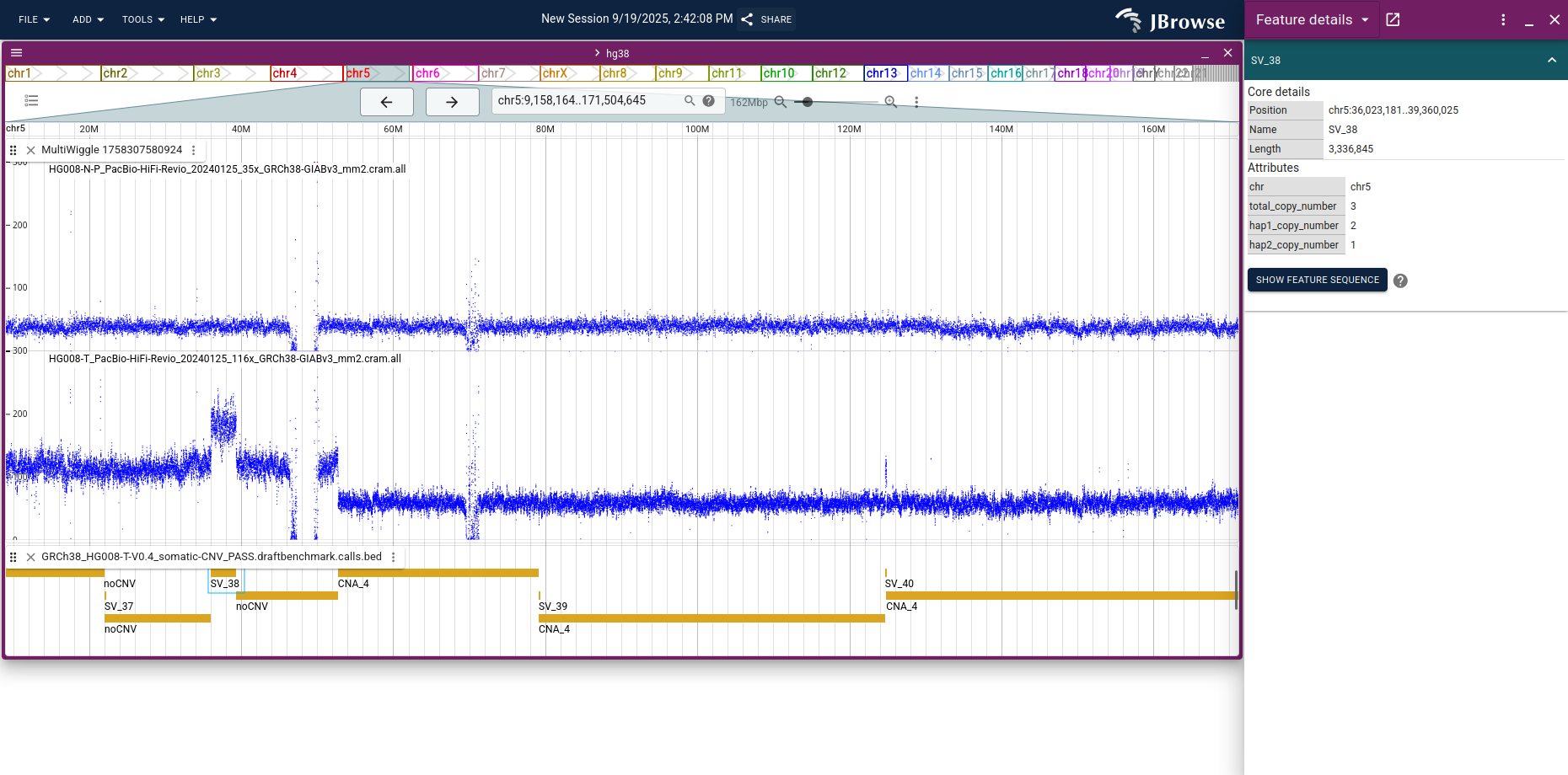
This protocol does not perform normalization or CNV calling; the bigWig view is a sanity check on existing calls, not a substitute for a CNV caller. See the multi-quantitative track guide for more on tumor vs normal coverage comparison.

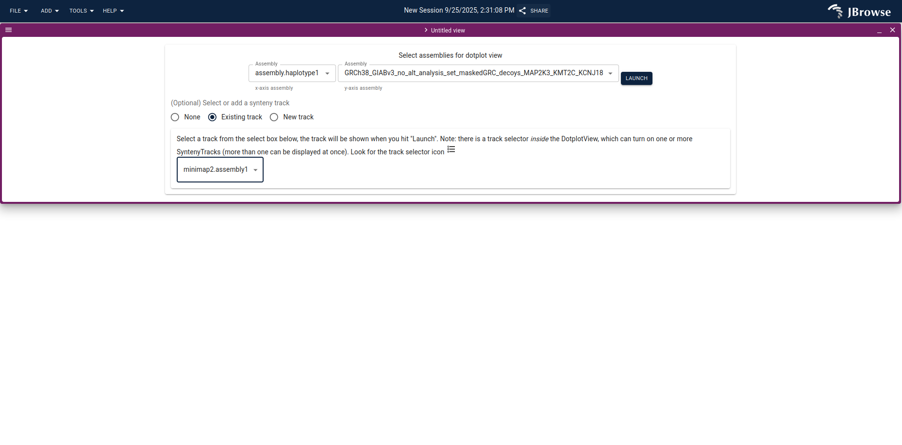
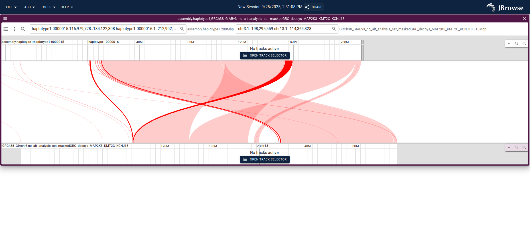
Walkthrough: synteny and dotplot views of the tumor assembly

Showing the tumor assembly side-by-side with the reference often makes complex SVs much easier to read than the alignment track alone. Open a dotplot view from the start screen, set the de novo assembly as one axis and GRCh38 as the other, and pick the matching synteny track.

The dotplot import form, with the HG008-T hap1 assembly on one axis and GRCh38 on the other.

The resulting dotplot reveals chromosomal rearrangements as off-diagonal segments — for example, the chr3 ↔ chr13 fusion shown in the SV inspector walkthrough above appears as a distinctive off-diagonal block.

The resulting dotplot, showing chromosome-scale rearrangements. The chr3–chr13 fusion from the earlier walkthrough is visible as an off-diagonal block.

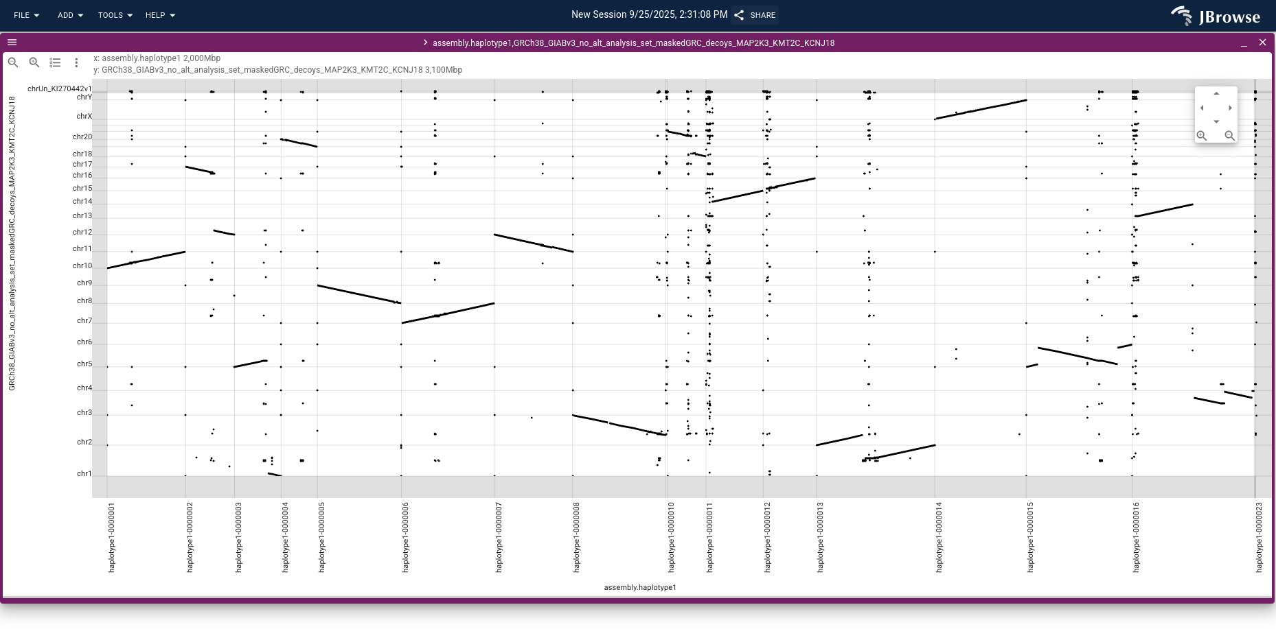
Click and drag over the rearranged region and choose Launch synteny view to see a base-level alignment of the two genomes; entering chr3 chr13 in the GRCh38 search box focuses the view on just those chromosomes.

A synteny view launched by selecting the chr3/chr13 region in the dotplot — base-level alignment makes the breakpoints easy to read.

For more on these views, see the dotplot view guide and the linear synteny view guide.

See also: Synteny and genome alignment — a complementary tutorial on comparing genome assemblies using the same views.

Troubleshooting

Problem	Possible cause	Solution
The browser stalls when viewing SV regions	Too large a region is being loaded with full alignment data	Use the Force Load option with care; downsample very high-depth data; or pre-filter to informative reads (e.g. discordant pairs, split reads with the SA tag)
The view is blank, or every position looks like a SNP	Data was aligned to a different reference than the loaded assembly	Make sure the BAM/CRAM/VCF were aligned against the same FASTA loaded into JBrowse
The synteny or dotplot view is blank	The assembly arguments to add-track -a are flipped	If you ran minimap2 ref.fa query.fa > out.paf, then load with jbrowse add-track -a query,ref — the order matters
Errors involving Node.js, or the wrong Node.js version is installed	The apt repository ships an older Node.js	Run sudo apt-get purge -y nodejs npm, then install from nodejs.org or NodeSource

If you hit a problem not covered above, please file an issue on the JBrowse 2 GitHub repository.

Next steps

Now that you've explored the C-GIAB HG008 dataset, you can:

• Load your own SV data — replace the C-GIAB VCF and BAM files with your own calls and sequencing data. The same workflows apply; the main difference is that your dataset may have different characteristics (e.g., smaller deletions, germline calls, SNVs instead of SVs).
• Customize track displays — try different color schemes (pair orientation, insert size), read filtering (discordant pairs, soft-clipped), and display modes (pileup, read arc, linked reads) to find the visualization that best highlights your findings.
• Use JBrowse Desktop — all of these workflows work identically in JBrowse 2 Desktop (Mac, Windows, Linux), which can load files from your local machine without needing a web server.
• Design a de novo assembly alignment — if you have a phased or haplotype-resolved assembly of your own sample, follow the minimap2 steps above to create a dotplot and synteny view.

For more on customizing JBrowse 2, see the SV visualization guide.

References

Diesh, C., Stevens, G. J., Xie, P., et al. (2023). JBrowse 2: A Modular Genome Browser with Views of Synteny and Structural Variation. Genome Biology, 24(1), 74.

McDaniel, J. H., Patel, V., Olson, N. D., et al. (2025). Development and Extensive Sequencing of a Broadly-Consented Genome in a Bottle Matched Tumor-Normal Pair. Scientific Data, 12(1), 1–22.

Rautiainen, M., Nurk, S., Walenz, B. P., et al. (2023). Verkko: telomere-to-telomere assembly of diploid chromosomes. Nature Biotechnology, 41(6), 753–762.

Data availability

Raw data from C-GIAB is under NCBI BioProject PRJNA200694. Processed data and benchmark call sets are available from the NIST Cancer Genome in a Bottle page. For the methods behind the dataset, see McDaniel et al. 2025.